Tutorials¶

FANFARE is best run in a jupyter notebook and below are examples of what can be done with the provided notebooks.

To open and run a tutorial, go to the main directory of FANFARE (where the *.ipynb files are) and type

ipython notebook

or

jupyter notebook

0. Creating a new dataset¶

See the notebook Tutorial 0 - Creating a new dataset.ipynb

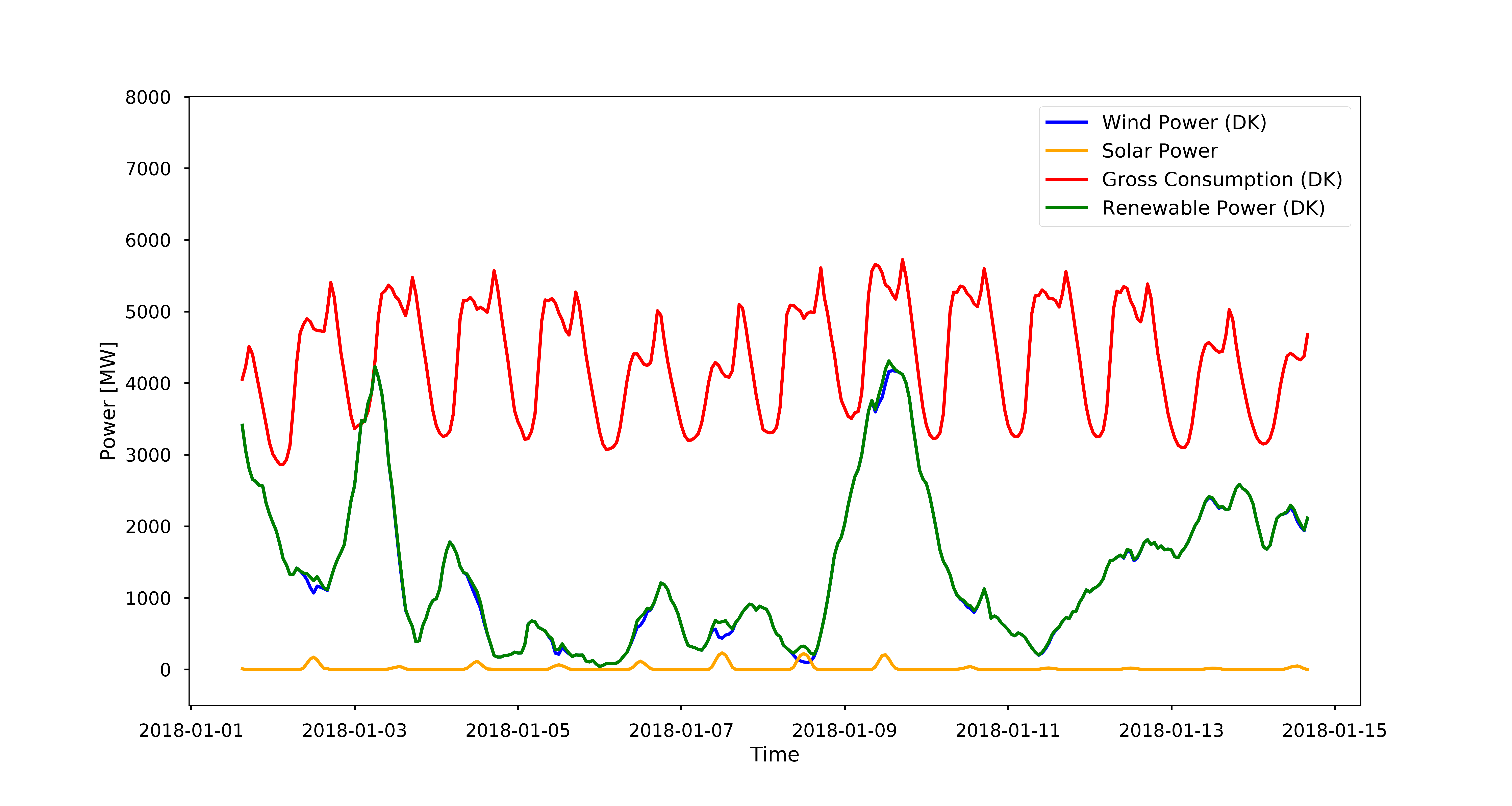
By going through the steps in this notebook, you should be able to generate the following plot with data from energidataservice.dk (Energinet data):

2. i) Oscillation analysis of residual load¶

See the notebook Tutorial 2 - i) Oscillation analysis of residual load.ipynb

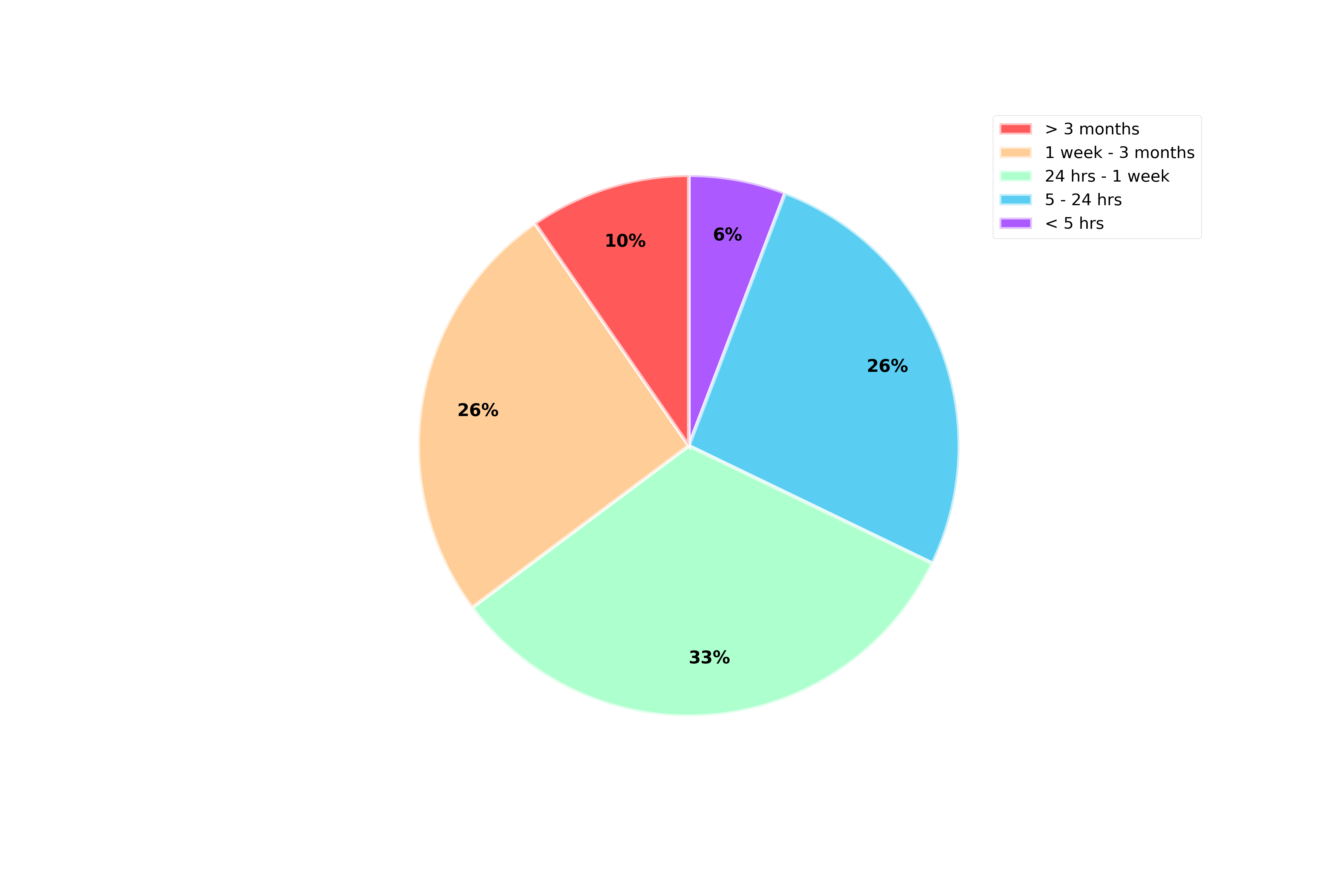
This is option (i) of the FANFARE method (see frontpage), where the discrete Fourier transform (DFT) is calculated and split into different freqency intervals, and the resulting iDFTs of each interval is integrated. In this notebook, you get to chose the frequency intervals of interest and make a pie chart displaying the energy stored in each interval:

3. ii) Power requirements from DFT analysis¶

See the notebook Tutorial 3 - ii) Power requirements from DFT analysis.ipynb

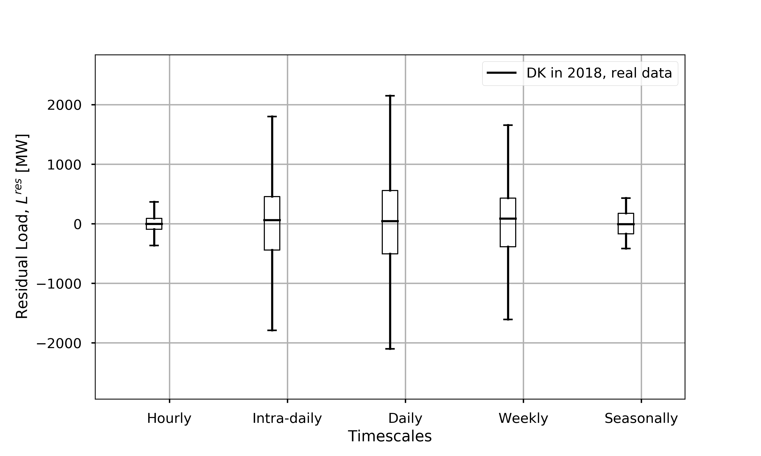
This is option (ii) of the FANFARE method (see frontpage), where the spread in residual load whithin each frequency interval is investigated.

4. iii) Storage capacity requirements from DFT analysis¶

See the notebook Tutorial 4 - iii) Storage capacity requirements from DFT analysis.ipynb

This is option (iii) of the FANFARE method (see frontpage), where a cumulative sum of the residual load whithin each frequency interval is used to place requirements on the storage capacity for those timescales.

Capacity requirements:
For frequency cut 0: 1.89e+00 GWh
For frequency cut 1: 2.11e+01 GWh
For frequency cut 2: 1.18e+02 GWh
For frequency cut 3: 4.20e+02 GWh
For frequency cut 4: 8.27e+02 GWh

Tutorials¶

0. Creating a new dataset¶

1. Hourly share of VRE in dataset¶

2. i) Oscillation analysis of residual load¶

3. ii) Power requirements from DFT analysis¶

4. iii) Storage capacity requirements from DFT analysis¶